From Brownian Motion to DDPM: The Origin and Elegance of the Diffusion Noise Formula
Introduction
Denoising Diffusion Probabilistic Models (DDPMs) have achieved astonishing success in image generation. Their core idea is very simple: gradually add noise to the data until it becomes pure noise, then learn the reverse denoising process to recover the data from noise.
But if you look closely at the forward diffusion process, you will find that it is not simply adding random noise to the data. Instead, it uses a very special weighted form:
where $\beta_t \in (0,1)$ is a small constant representing the “noise strength” at each step.
This formula may look like it simply “shrinks the signal a little, then adds a little noise,” but why are the coefficients specifically $\sqrt{1-\beta_t}$ and $\sqrt{\beta_t}$? Why not write it directly as $x_t = x_{t-1} + \sqrt{\beta_t}\varepsilon_t$? Or why not $x_t = (1-\beta_t)x_{t-1} + \beta_t \varepsilon_t$?
This article traces the origin of the formula back to the Ornstein-Uhlenbeck process in nonequilibrium statistical physics, derives the original discrete form of the DDPM forward process, and then shows how the constraints of variance preservation and Taylor approximation eventually lead to the elegant expression you see today. We will also see how this ingenious design makes the entire reverse diffusion process highly tractable and ultimately condenses into an extremely simple “predict the noise” training objective.
1. Physical Origin: The Ornstein-Uhlenbeck Process
The idea behind DDPM can be traced back to the work of Sohl-Dickstein and others in 2015, where they drew inspiration from diffusion processes in nonequilibrium thermodynamics. In physics, a classic model is the Ornstein-Uhlenbeck (OU) process, which describes the velocity evolution of a particle in a viscous fluid: the particle is affected both by friction, which causes its velocity to decay, and by random thermal collisions from surrounding molecules, which produce random perturbations.
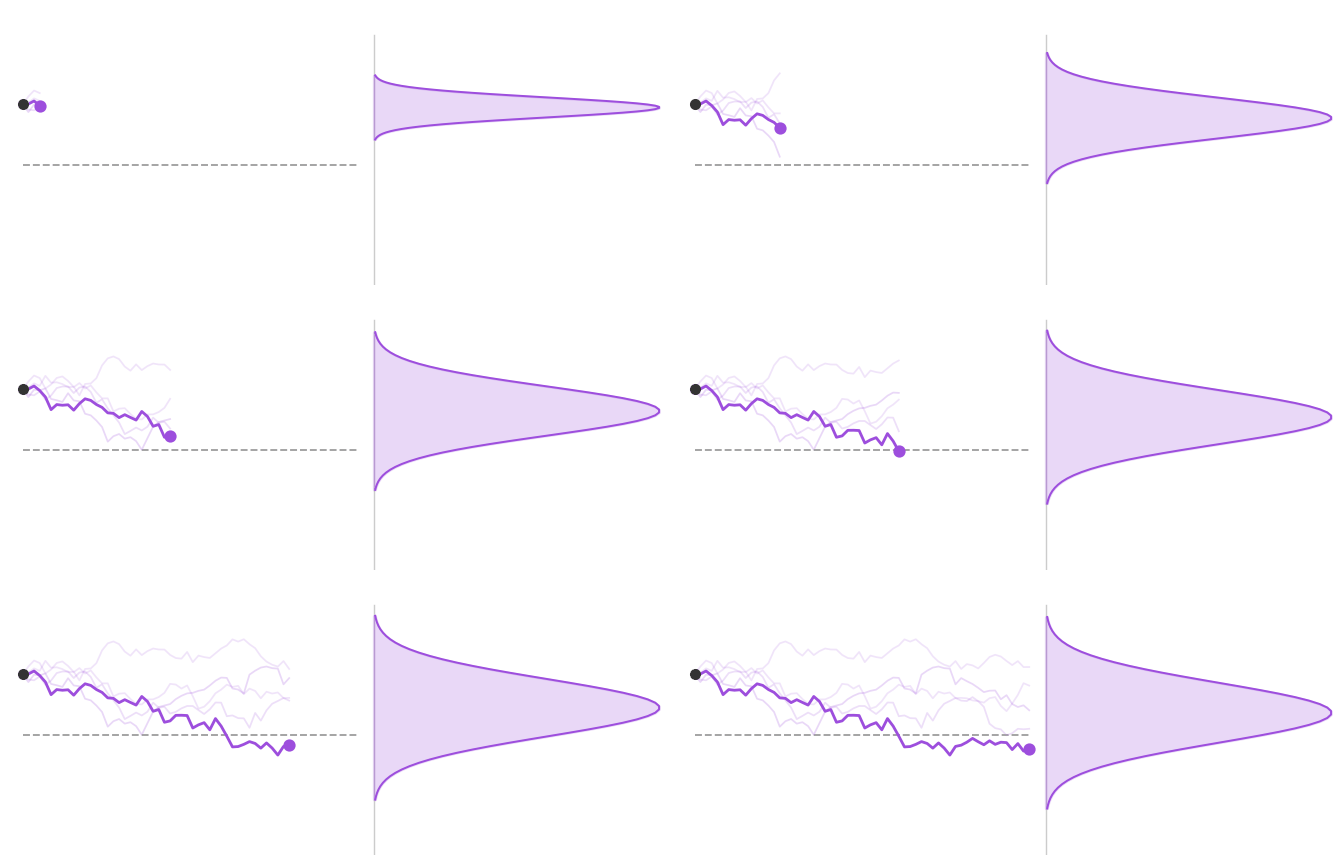
The OU process is described by a stochastic differential equation (SDE):
- $x$ is the system state, such as velocity.
- $-\theta x \, dt$ is the drift term; $\theta > 0$ is the relaxation rate, which pulls $x$ toward zero mean and represents energy dissipation.
- $\sigma \, dw$ is the diffusion term; $dw$ is the increment of a Wiener process (white noise), satisfying $dw \sim \mathcal{N}(0, dt)$.
The solution of this equation converges, in the long-time limit, to a stable Gaussian distribution $\mathcal{N}(0, \sigma^2 / (2\theta))$. This is the physical prototype of a diffusion process from “order to disorder.”
2. Toward DDPM: Variance-Preserving SDE (VP-SDE)
The goal of DDPM is not to simulate an arbitrary physical process, but to gradually transform an arbitrary data distribution into standard Gaussian noise $\mathcal{N}(0, \mathbf{I})$, while keeping the signal scale at each intermediate step approximately constant to ensure numerical stability. This requires a special choice of parameters in equation (2).
To make the final variance equal to 1, we can choose the parameters as follows: let $\theta = \frac{1}{2}\beta(t)$ and $\sigma = \sqrt{\beta(t)}$, where $\beta(t) > 0$ is a slowly varying function of time, i.e. the noise schedule. Substituting into equation (2) gives:
This is the well-known Variance Preserving SDE (VP-SDE), the continuous-time version of DDPM. It can be shown that when the initial variance is 1, the marginal variance of this SDE remains exactly 1 at all times and converges to $\mathcal{N}(0, \mathbf{I})$ as $t \to \infty$.
3. Discretization: The Discrete Recurrence of the OU Process
To implement this on a computer, we need to discretize the continuous-time SDE (3). Set the discrete step size $\Delta t = 1$, and let $\beta_t = \beta(t) \Delta t$. Using the most direct Euler-Maruyama discretization:
- Drift term: $-\frac{1}{2}\beta(t) x \, dt \;\longrightarrow\; -\frac{1}{2}\beta_t \, x_{t-1} \cdot \Delta t = -\frac{1}{2}\beta_t x_{t-1}$
- Diffusion term: $\sqrt{\beta(t)} \, dw \;\longrightarrow\; \sqrt{\beta_t} \, \varepsilon_t \sqrt{\Delta t} = \sqrt{\beta_t} \varepsilon_t$, where $\varepsilon_t \sim \mathcal{N}(0, \mathbf{I})$
Thus SDE (3) becomes the discrete recurrence:
Rearranging gives:
This is the original noise-addition formula obtained directly by discretizing the physical OU process. It is the earliest form of the DDPM noising mechanism.
4. The Approximation Revealed by Taylor Expansion
Notice that the scaling coefficient in equation (4) is $1 - \frac{1}{2}\beta_t$, while DDPM ultimately uses $\sqrt{1-\beta_t}$. What is the relationship between them? The answer lies in the first-order Taylor expansion.
Consider the function $f(\beta) = \sqrt{1 - \beta}$. Its Maclaurin expansion at $\beta = 0$ is:
Compute: $f(0) = 1$, $f'(\beta) = -\frac{1}{2\sqrt{1-\eta}}$, so $f'(0) = -\frac{1}{2}$. Therefore:
When $\beta_t$ is very small, for example on the order of $10^{-4}$ to $10^{-2}$, the higher-order term $\mathcal{O}(\beta_t^2)$ can be ignored, so:
This means that in the small-noise limit, the OU discrete formula (4) and the final DDPM formula (1) are almost identical. But the authors of DDPM did not stop at this approximation; they made a crucial theoretical leap.
5. Perfect Variance Preservation: From Approximation to Exactness
If $\sqrt{1-\eta_t}$ can replace $1 - \beta_t/2$, why go to the trouble? The reason is exact variance conservation.
Assume the variance of $x_{t-1}$ is $\text{Var}(x_{t-1}) = 1$. Let us compute how the variance changes under the two recurrences.
For the OU discretization (4):
The variance gains a tiny increment of $\beta_t^2/4$. Although this is very small in a single step, after accumulating over thousands of steps, the variance will gradually drift, causing the distribution of $x_T$ to deviate from $\mathcal{N}(0, \mathbf{I})$, and the scale of intermediate-layer inputs will no longer remain stable.
For DDPM's $\sqrt{1-\beta_t}$ in (1):
The variance is exactly locked to 1! No matter how many steps are taken, as long as the initial variance is 1, the marginal variance of $x_t$ at each step remains strictly constant. This is where the name “Variance Preserving” comes from.
Therefore, DDPM's choice of $\sqrt{1-\beta_t}$ is not a casual approximation, but an ingenious construction that makes the variance identity hold exactly in mathematics. It perfectly inherits the first-order behavior of the OU process discretization while achieving absolute precision in numerical stability.
6. Reparameterization: The Elegance of a One-Step Form
Another major strength of the DDPM forward formula is that it can be reparameterized. Let $\alpha_t = 1 - \beta_t$ and $\bar{\alpha}_t = \prod_{s=1}^t \alpha_s$. Repeatedly applying equation (1) and using the closure of the Gaussian distribution yields:
This means that the noisy sample at any time step $t$ can be sampled directly from the original data $x_0$ in one step, without any iterative procedure! This is a huge efficiency gain for training, because we only need to randomly sample a timestep $t$ and can immediately compute $x_t$ as the network input.
At the same time, when $t \to T$ is sufficiently large, $\bar{\alpha}_T \to 0$, so $x_T \to \mathcal{N}(0, \mathbf{I})$, perfectly converging to the prior distribution.
7. Reverse Process and the Simplification of the Training Objective
The clever design of the forward process directly determines that the reverse denoising process also has an extremely simple form.
Given $x_t$ and $x_0$, the reverse conditional probability $q(x_{t-1} | x_t, x_0)$ is also Gaussian, and its mean can be written exactly as:
Using the reparameterization in equation (5), solve for $x_0 = \frac{1}{\sqrt{\bar{\alpha}_t}}(x_t - \sqrt{1 - \bar{\alpha}_t} \bar{\varepsilon})$. Substituting this in reveals that the mean $\tilde{\mu}_t$ actually only needs the prediction of the noise component $\bar{\varepsilon}$ that we added. Therefore, we can train a neural network $\varepsilon_\theta(x_t, t)$ to predict the noise and construct the reverse sampling step:
After a series of simplifications, the variational lower bound (ELBO) of DDPM ultimately yields a surprisingly simple loss function:
The training objective is simply to let the model accurately guess the Gaussian noise $\varepsilon$ that was originally mixed in, given the noised sample $x_t$ and the timestep $t$. No adversarial training, no complicated variational tricks, just a plain mean-squared-error regression.
Conclusion: The Multiple Layers of Wisdom Behind One Formula
Looking back over the whole derivation, the DDPM noise-addition formula:
is by no means made up out of thin air. It embodies multiple layers of deep insight:
- Physical inheritance: It comes from the Euler discretization of the Ornstein-Uhlenbeck process and naturally carries the thermodynamic essence of “gradually diffusing into disorder.”
- Unifying approximation and exactness: Through the first-order Taylor approximation $1 - \beta_t/2 \approx \sqrt{1-\eta_t}$, it is equivalent to the physical discretization under small noise, while also achieving strict variance conservation and ensuring long-term numerical stability.
- Analytical tractability: The variance-preserving construction gives the forward process perfect reparameterization properties, so any intermediate distribution can be sampled in one step, and the reverse conditional distribution is Gaussian with a closed-form solution.
- Extreme simplification of training: The final loss collapses to an L2 loss for noise prediction, making training exceptionally stable and easy to scale.
The “particular elegance” of this additive form is, at its core, a beautiful intersection of physics, probability theory, and numerical optimization. When you see this simple expression, remember the elegant derivation chain behind it: from Brownian motion, through stochastic differential equations, discretization, and Taylor expansion, all the way to exact variance preservation. It is this rigorous yet elegant design that laid the mathematical foundation for the large-scale success of diffusion models.